On the relevance of the probability distribution.

Some time ago, I had already presented some results on simple games. Now, a friend of mine has started to trade and I want to help him understand something.

Imagine you have a game where you bet 100 and can get either 110 or 90 with 50% probability. 

Suppose you play this game 200 times and in each game you bet a fraction f (0<f<1) of your whole equity. What happens to your equity after 200 games?

The simple answer is: you get the initial equity because you win 10 or lose 10 with equal probability. But a more detailed answer is given in the next figure, which shows a simulation of 100k experiments:

As there are probabilities involved, we only can get statistical results. The green line depicts the mean value of the equity, which is 100 irrespective on the fraction that you bet. But the shades of blue also indicate the distribution! They are chosen so that the light blue area represents 90% of the population and so on, as given in the legend. The blue line represents the median: the separation between the top 50% and the bottom 50%. (The frontiers between shades of blue are the percentiles 95, 87.5, 75, 62.5, 50, 37.5, 25, 12.5 and 5)

So, the interesting thing is that even if the mean is 100, in 75% of the experiments your final equity is less than the initial one if you bet your full equity (f=1). If you bet 40% of your equity (f=0.4) you are under the mean only in 62.5% of the cases.

So, be careful with the probability distribution of your equity. The mean may look important, but is meaningless in these long tailed cases!

A Losing Strategy?

A given strategy gives you x1.2 your original investment 50% of the time and x0.822 your original investment 50% of the time.Note that 1.2·0.822 = 0.98623 which is less than one. So, if you trade this system 100 times with your full equity, assuming you get 50 winning and 50 losing trades, your will end up with a 50% loss, as 1.2^50*0.822^50=0.5.

This is not appealing, is it? But, what happens if you always trade a fraction "f" of your current equity? Look a the graph below, showing the simulated results for 10k experiments:

As in this post, the blue shaded areas correspond to areas including 25%, (darkest), 50%, 75% and 90% (lightest) of the outcomes. The frontiers between areas are 5%, 12.5%, 25%, 37.5%, 62.5%, 75%, 87.5% and 90% percentiles. The solid blue line corresponds to the theoretical case: half of the results lie above and half below this line. The green line is the mean of the outcomes.

It follows, that you may get a final equity E, greater than the initial one Eo. Specifically E>1.016·Eo in 62.5% of the cases if you make each trade with f=0.1, i.e. 10% of our equity.

The following simulation is a similar case where the gains are x1.5 and x0.6575:

Clearly, this might be attractive, depending on your level of risk!

What quantity should I trade?

Problem Outline

Let's suppose you have developed a trading system. On average, 50% of the trades give you a 10% profit and 50% of the trades give you a 5% loss. 

The Theory

Suppose that you have an initial account of 100 and you make 50 trades. In each trade you invest your total equity. In theory, 25 trades would increase your equity by a factor 1.1, and 25 trades would decrease it by a factor 0.95. So, the net result should be

E  =  Eo·1.1^25·0.95^25  =  Eo·3

So, your final equity would be 3 times your initial equity Eo.

What happens if you invest a fraction f (0<f<1) of your equity in each trade? On each trade you take f away and you recover f*1.1 or f*0.95. Assuming 25 successful and 25 unsuccessful trades, you end up with

E(f)  =  Eo·(1-f+f*1.1)^25 ·(1-f+f*0.95)^25

Simulation of Real Cases

What happens in practice? I have made some simulations of trading sequences. Random numbers between 0 and 1 are generated. If they are > 0.5, we assume a gain of 1.1, else a loss of 0.95.  Figure 1 shows the resulting equity after 50 trades for different values of f.

Figure 1

The green line is the theory discussed above, the blue line is the mean of 1000 experiments. There is a reasonable agreement. In addition, the plot shows a filled area, which corresponds to the mean plus minus one standard deviation. The dashed green lines correspond to the theoretical case, but with 55% gains and 45% losses and vice-versa.

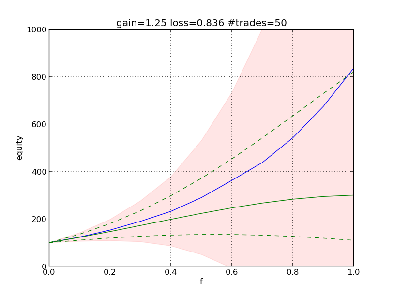
What happens if we change the gain (pg) and loss (pl) levels? Figure 2 shows the results of a simulation for pg=1.25, pl=0.836 for 50 trades. To get a smoother curve, this has been done for 10k experiments.

Figure 2

The green line is, again, the theory. Trading the full account (f=1) this gives the same theoretical result E=Eo·3 as before. The green curve is, however quite flat, suggesting that, we may trade smaller amounts with similar result.

Observe the green dashed lines, obtained as before. If a specific run has 55% losses, instead of 50%, and we are trading with f=1, we will end up with E=Eo·1.1.

It seems also surprising that the blue line, the mean of 10k experiments, looks so much "better" than the theory. This may be explained because there is a lower limit of 0.836^50, i.e. 0 for practical purposes and an upper limit of >70000. Note that we have a distribution that is not normal (in the statistical sense).

The coloured area may be misleading, suggesting negative outcomes. Keep in mind that it is only a representation of the standard deviation of the blue line. For f=1 the mean is 838 and the standard deviation is 2167!

More meaningful results are obtained from the plot in Figure 3. Here, I have added blue dotted lines corresponding to the percentiles 5%, 15%, 25% 50%, 75%, 85% and 95%.

Figure 3. Blue dotted lines at 5%, 15%, 25% 50%, 

75%, 85% and 95% percentiles

We may observe that the percentile 50% line falls exactly on the green (theoretical) line. We also observe that there is roughly a 20% chance that we end up losing money (E<100) with this technique when f=1.

Some interesting conclusions:

• If we want to trade with this technique and we want be sure that we do NOT lose money in 95% of the cases, we should NOT trade. This is indicated by the maximum of the lowest dotted line being at f=0
• If we want to maximize our return in 75% of the cases, we should invest at the maximum of the third dotted line, which happens at f=0.65 

Discussion

1) The simulation of real cases (there is some irony in this!) shows that reality is quite different from the theory. The case discussed in the first chapter of The Mathematics of Money Management by Ralph Vince, showing a nice and sharp maximum for f=0.25, only happens for games with extreme gain (and loss) values, which we are unlikely to find in trading.

2) The results are very sensitive if gains and losses are big and small, respectivelly. To achieve a theoretical final value E=Eo·3 for pg=1.5, we need

pl=3^(1/25)/1.5=0.69662

But, if we use two decimal positions and compute 1.5^25·0.69^25 we get E=Eo·2.34, and 1.5^25·0.69^25 gives E=Eo·3.38

3) Mean and standard deviation are useless measures if the distribution is not normal. Percentiles give more information. In our case, the theoretical case corresponds to the 50% percentile.

Some "Equivalent" Systems

Next are the simulation plots for some systems with pg·pl=1, which are theoretically equivalent if traded with f=1: they all give E=Eo after 100 trades. There are, however significant differences between them!

 Figure 4

 Figure 5

Figure 6

In these plots, the blue shaded areas correspond to areas including 25%, (darkest), 50%, 75% and 90% (lightest) of outcomes. The frontiers between areas are 5%, 12.5%, 25%, 37.5%, 62.5%, 75%, 87.5% and 90% percentiles. The solid blue line corresponds to the theoretical case: half of the results lie above and half below this line. The green line is the mean of the outcomes. The long tails of the resulting distribution are responsible for the upward bias, but this is nevertheless, the real mean!

So, if you were offered one of these three systems, what would you do? You could elect the first one, where pg=1.3 and pl=0.77. Trading using this system with f=0.3 you will obtain E>1.25·Eo in 75% of the occasions. Do NOT trade this system with f=1!